Annotation

1 Overview

This document describes the preliminary SeaBee annotation workflow for habitat mapping. The aim of these notes is to help new users get started with annotation using ArcGIS Pro and to avoid common mistakes/pitfalls.

2 Workflow

2.1 Install ArcGIS Pro

Follow the steps below to download and install ArcGIS Pro on your local machine.

Contact Debhasish Bhakta to obtain login details for ArcGIS Online. You need access to ArcGIS Pro with the Image Analyst extension.
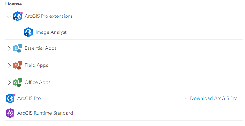
Login to ArcGIS Online and, under your profile, choose Settings > Licenses. Check that Image Analyst is available to you under ArcGIS Pro extensions, then click the link to Download ArcGIS Pro (Figure 1).
Obtain an administrator password from IT-Vakt and run the installer. You should then be able to start ArcGIS Pro and login to the application using your ArcGIS Online credentials.

2.2 Setup project

The next step is to create a new project within ArcGIS and add SeaBee data to it.

In ArcGIS Pro, create a new Map project. The Name should describe the mission/area you’re annotating and Location should be an existing local folder on your PC.

Tip

ArcGIS may run slowly if you set Location to be a network folder or a folder that is synchronised to an external server (e.g. DropBox, OneDrive, GoogleDrive).

Within your project folder, create three new subfolders: class_definitions, vector and raster. This can either be done using the Catalog pane in ArcGIS or using Windows’ File Explorer.
Download relevant mission datasets and add them to the appropriate subfolders. As a minimum, you will need a class definition file, a georeferenced orthomosaic (or WMS layer) and a region of interest (ROI) file. Optionally, you may include a ground truth dataset and any pre-existing annotation for your area of interest. See Section 2.3 to Section 2.6 for details.

2.3 Class definition files

ArcGIS Pro supports hierarchical class definitions, which can be defined manually via the Training Samples Manager. Class definitions are saved as ESRI Classification Schema files (.ecs), which are JSON files with a specific structure.

The classes of interest to SeaBee are complex and creating them manually via the user interface is cumbersome. Section 2 of the notebook here includes code to build an .ecs file with the correct schema from an Excel table, which is more convenient in most cases.

As far as possible, SeaBee will use a standard set of class definitions for habitat mapping. The latest versions are available online here in both Excel and .ecs formats.

The workflow for class definition files is as follows:

Before starting to annotate a new area, everyone involved must agree on which set of class definitions (i.e. which version) to use. If necessary, class definitions can be updated in Excel and a new version of the .ecs file created using the code linked above.
Everyone should download the same .ecs file and add it to the class_definitions folder in their ArcGIS project (created in Section 2.2).

Important

Using a standard set of classes is important if the machine learning algorithms created by SeaBee are to be transferable/re-trainable. It is likely that some changes to the class schema will be necessary initially, but we are hoping to converge on a standard set of habitat classes if possible. Proposed changes should be discussed with Hege Gundersen and Kristina Øie Kvile.

2.4 Orthomosaics

Orthomosaics for your area of interest should be added to your map. You can either download them via MinIO and add them to the raster folder within your ArcGIS project, or connect to the SeaBee WMS and add them as web service layers. In most cases, the RGB mosaics are most useful for annotation, since they look familiar and have the highest resolution. Multispectral data may be worth including in some cases, although it has not been used much for annotation so far.

Tip

Downloading large files from MinIO can be slow and unstable. If you wish to store the data locally, consider using RClone. Using WMS layers is generally easier, but unfortunately they are not recognised by Image Analyst. If you wish to use the WMS, you will need to add at least one local raster file to your map covering your area of interest.

2.5 Ground truth data

Point shapefiles of ground truth data are available for most missions. These are typically stored in the mission folders on MinIO within subfolders called ground-truth, or at a higher level find the folder structure (e.g. a single ground truth dataset for an entire SeaBee campaign).

If available, download the shapefile and add it to the vector folder within your in ArcGIS project.

2.6 Region of interest and training subareas

For each mission, you should create shapefiles defining (i) your region of interest (ROI), and (ii) a set of subareas that will be used to divide the annotation data into “blocks”. When you create these shapefiles, be sure to use the same co-ordinate reference system (CRS) as the orthomosaic you wish to annotate.

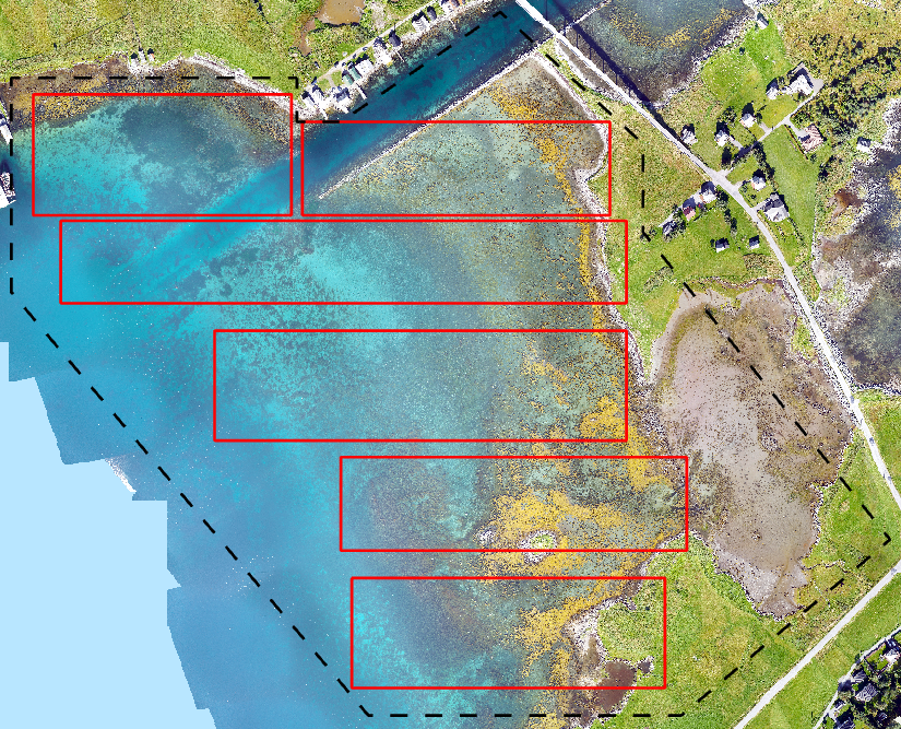
The ROI defines the area that you would eventually like to classify. This will typically cover a large proportion of the total image, but excluding anything not covered by your class definition file (see Section 2.3). As an example, see the black dashed line defining the ROI for Remøy on Figure 2.

Machine learning algorithms only learn based on the training samples you provide, so if the prediction area includes things not present in the training data you will get poor results. If possible, use the ROI file to define an area excluding things like roads, buildings and bridges that you are not interested in. You can then ignore these at the annotation stage and focus instead on annotating classes of ecological interest.

Important

If your area includes lots of man-made objects and you can’t exclude them using an ROI for some reason, make sure you annotate a representative selection of each type of object and tag them all as ANTHRO.

The training subareas are a set of rectangles (say, 1 to 10) that define discrete areas within which you create annotation. See the red rectangles on Figure 2 for an example from Remøy. Defining subareas is helpful because we might want to train an algorithm using annotations from e.g. Areas 1 to 3, then iteratively evaluate it against data from Areas 4 and 5. Once we’re satisfied, we can use data from Area 6 to get a independent assessment of the model’s performance.

Defining training subareas is also a convenient way of dividing the annotation workload between several people: each person agrees to annotate one or two specific subareas. This avoids accidental duplication of effort (although at times it may also be useful for several people to annotate the same area to assess consistency).

Figure 2: Region of interest and training subareas used for Remøy

If you do not wish to use subareas, simply create files named roi.shp and subarea_bounds.shp and add a single polygon to each defining the area to be annotated.

2.7 Styling the map

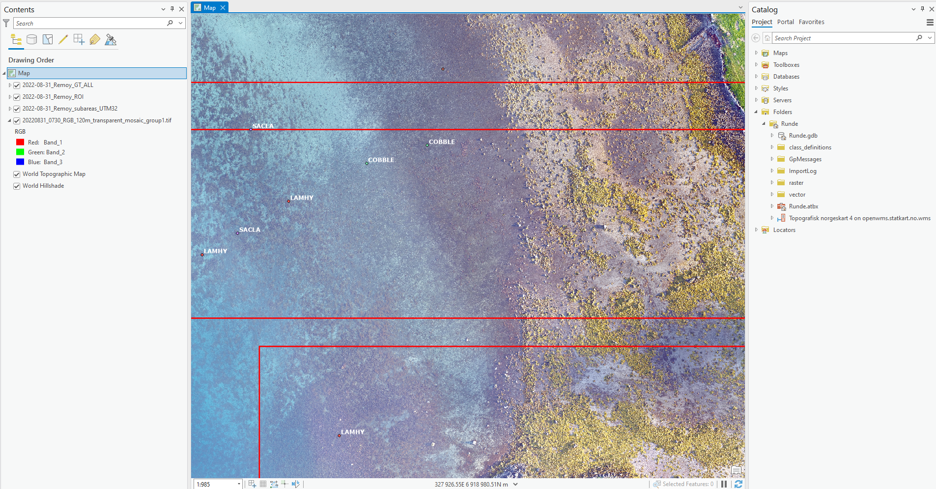
Once you have download all the relevant datasets and added them to your project folder in ArcGIS, you can add layers to your map and style them appropriately. Figure 3 shows an example.

Drag each layer from the Catalog pane (right-most column in Figure 3) to the ArcGIS Table of contents (left-most pane in Figure 3). The order of layers in the Table of contents defines the drawing order on the map, so put the orthomosaic at the bottom and the other layers on top.
Right-click each vector layer in the Table of contents and choose Symbology. This will allow you to define fill and outline colours for the vector layers on your map.
[Optional] Right-click the ground truth dataset and choose Labelling Properties. Set the Expression to be $feature.Kode, where Kode is the name of the column in the ground truth attribute table containing the labels you want to use. When you click Apply, you should see each point in the ground truth dataset labelled with its class code.

Tip

Whenever you’re working with anything GIS-related, remember to save your work regularly!

2.8 Creating annotation

With the ArcGIS project configured, you can begin creating annotation.

In the ArcGIS Table of contents (left-most pane in Figure 3), select one of your orthomosaic layers. This will activate the Image Analyst extension. Note that if you’re using WMS layers, these are not recognised by Image Analyst. In this case, select a local TIFF file for your area of interest and use this instead (see tip above).
On the “ribbon” (i.e. menu bar), select the Imagery tab and choose Classification Tools > Training Samples Manager. A new pane should appear at the right side of the window.
In the upper part of the new pane, click the folder icon (which has a tooltip saying Classification schema) and load your class definition file (see Section 2.3). You should see the class hierarchy added to the upper half of the window.
Identify the training area you wish to annotate and zoom in on a feature (e.g. a boulder or patch of algae). In the class hierarchy, select the class you wish to annotate, choose one of drawing tools from the top of the window and begin digitising. In most cases, the Freehand tool is likely to be most useful.

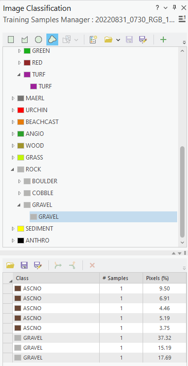
Each polygon you draw will appear in the lower half of the Image Classification pane (see Figure 4). The Pixels (%) column shows what proportion of the pixels digitised so far belong to each class.

It is a good idea to periodically group polygons of the same class. This is done by selecting the rows you wish to group in the lower pane (using SHIFT + Click or CTRL + Click) and then clicking the Collapse icon (two arrows coming together). You can also ungroup using the Expand button (one arrow splitting into two).
When you have finished your digitising session, click the Save icon in the lower pane of the Training Samples Manager to save your training samples as a shapefile in the vector folder of your ArcGIS project. You should also save the entire ArcGIS project before closing down.
If you wish to continue annotating using a shapefile created previously, first open your ArcGIS project and load the class definitions file (steps 1 to 3 above). Then, instead of creating new annotation from scratch, click the folder icon in the lower part of the Image Classification pane (labelled Load training samples) and browse to the annotation shapefile created previously. You can now continue annotating and save changes back to the original shapefile.

Tip

The following tips should help you to create good quality annotation:

Always assign the most detailed level in the class hierarchy that you can confidently identify. If you are not sure, assign the level above.
Group your polygons by class regularly and get into the habit of clicking Save immediately before each grouping operation.
Use the Pixels (%) column to prioritise which classes to focus on. Given the classes of interest, you will probably not be able to produce a “balanced” training dataset, but if you have e.g. 90% BOULDER there’s no point digitising more boulders.
You don’t need to digitise everything within each training subarea (but the more the better).
Do not annotate anything outside of the training subareas and do not draw polygons that cross subarea boundaries.
Do not draw overlapping polygons or polygons that touch one another (ideally, there should be at least one pixel between adjacent polygons).
Do not draw self-intersecting polygons (i.e. when the line you’re drawing crosses itself, such as when drawing a figure-of-eight or bow-tie shape). Such polygons are invalid and they cause problems later in the workflow. In particular, there is a bug/lack of error handling in ArcGIS Pro’s Training Samples Manager that causes the application to crash hard if you attempt to group invalid polygons.
If you’re not sure how to assign something, or where a boundary should be drawn, the key question to ask yourself is: “Would I be happy if an algorithm classified this entire polygon as X?” If the answer is “Yes”, it is reasonable to tag the whole polygon as X; if the answer is “No” consider subdividing or deleting it.

2.9 Packaging annotation

Once all subareas have been digitised, each person should upload their annotation shapefiles to MinIO using the following structure:

niva-tidy/annotation/
├─ campaign_year/
│  ├─ annotation_by_subarea
│  │  ├─ annotation_area1.shp
│  │  ├─ annotation_area1.shx
│  │  ├─ annotation_area1.dbf
│  │  ├─ annotation_area1.prj
│  │  ├─ annotation_area1.cpg
│  │  ├─ annotation_area2.shp
│  │  ├─ etc.
│  ├─ region_of_interest
│  │  ├─ roi.shp
│  │  ├─ roi.shx
│  │  ├─ roi.dbf
│  │  ├─ roi.prj
│  │  ├─ roi.cpg
│  ├─ subarea_boundaries
│  │  ├─ subarea_bounds.shp
│  │  ├─ subarea_bounds.shx
│  │  ├─ subarea_bounds.dbf
│  │  ├─ subarea_bounds.prj
│  │  ├─ subarea_bounds.cpg

Note the following:

campaign_year represents an entire campaign, which may involve multiple drone flights e.g. remoy_2022 or kelpmap_2022.
The folder annotation_by_subarea should contain one polygon shapefile per subarea. Make sure each subarea is included only once.
The region_of_interest subfolder should contain a single polygon shapefile defining the region of interest.
The subarea_boundaries subfolder should contain a single polygon shapefile with one polygon feature per subarea.

Once the data are uploaded to MinIO in the correct format, work through the notebook here. This will:

Merge the annotation shapefiles for each subarea into a single dataset.
Tag each of the annotation polygons with the subarea ID, making it easier to filter/subdivide the training data.
Reconstruct the original, three-column class hierarchy from the single-column ArcGIS output. This makes it easy to generate raster annotation for any of the three “levels”.
Create a geopackage combining the annotation data, the subarea polygons and the region of interest. The geopackage will be saved to MinIO in the campaign_year folder. This can then be shared with NR, together with links to the relevant orthomosaics.
Publish the annotation to GeoNode, using the same colour schemes as defined in the Excel templates and .ecs files.